Chapter 5 Parametric Equations & Curves
Section 5.1 Parametric Equations
Parametric equations can be used to caluculate the components of the points along a cuve as a function of an independent variable (commonly referred to as \(t\)). For example, let’s say we want to draw a line from \((x_0, y_0)\) to \((x_1, y_1)\text{.}\) We can define this parametrically as:
\begin{equation*}
\begin{aligned}
x \amp= x_0 + (x_1 - x_0)t \\
y \amp= y_0 + (y_1 - y_0)t
\end{aligned}
\end{equation*}
At \(t = 0\text{,}\) we just get \((x_0, y_0)\) and at \(t = 1\text{,}\) we get \((x_1, y_1)\text{.}\) As \(t\) moves over the range \(0\rightarrow1\text{,}\) these equations will generate all the points along the line. We already have a very good way of drawing a line, but we can generalize this process for other shapes, assuming we have functions \(f(t)\) which returns x values and \(g(t)\) which returns y values:
\begin{equation*}
\begin{aligned}
t \amp: 0\rightarrow1 \\
x \amp= f(t) \\
y \amp= g(t)
\end{aligned}
\end{equation*}
By using the framework above to generate points that we can add to our edge matrices, we can draw any shape that can be defined in such a manner.
Subsection 5.1.1 Parametric Circle
If you wanted to use this technique to draw a circle with radius \(r\) and center \((c_x, c_y)\text{:}\)
\begin{equation*}
\begin{aligned}
t \amp: 0\rightarrow1 \\
x \amp= rcos(2\pi t) + c_x \\
y \amp= rsin(2\pi t) + c_y
\end{aligned}
\end{equation*}
Section 5.2 Splines
Splines are a special set of polynomial curves. They are designed in such a way that you can combine 2 or more splines smoothly in order to generate higher degree curves. You may recall the term spline 1 from your drafting days, using splines to make non-arc based curves. In Computer Graphics, splines are an effective way of generating arbitrary curves effeciently. We will only need to create 3rd degree curves at most, but still be able to generate more complex looking ones by combining splines.
Remember that our purpose is to make a graphics engine, and not a graphing calcuator. So when thinking about drawing arbitrary polynomials, we have to think about what information is useful to us. Think about a circle, in order to draw one, we would like to know the center and radius. Turns out, that information not only describes the shape we’re drawing, but also goes directly into the parametric equations for making a circle. It is also easy to provide that information via a GUI (click center, drag for radius, boom). A standard 3rd degree polynomial, \(ax^3 + bx^2 + cx + d\) doesn’t trasnlate as easily into the graphical world. Think about drawing a line, we specify endpoints and generate the equation based on that. We will look at two types of splines, Hermite and Bezier curves, which are similar (in fact, you can translate between the two), but differ in the information required to generate a cruve.
Subsection 5.2.1 Hermite Curves
To generate Hermite Curves, we will need the following information:
- \(P_0, P_1\text{:}\) endpoints
- \(R_0, R_1\text{:}\) rates of change at each endpoint.
\(P_0, P_1\) designate where the curve starts and ends. Specifying rates of change at each endpoint allows us to both generate curves between the endpoints, but also connect multiple curves smoothly. Two Hermite curves that share a common endpoint and rate of change at that endpoint will nicely connect to create a larger, more complex cure.
We will use parametric equations to help get from this information to points along a curve, assuming \(t: 0 \rightarrow 1\text{:}\)
\begin{equation*}
f(t) = at^3 + bt^2 + ct + d
\end{equation*}
This is a standard cubic equation. Substituting for \(t\) will generate points along our curve. Ultimately, this is the equation we need to make a curve, so we will need to calculate the coeficients based on the given information.
In order to actually make a curve, we will need separate functions for \(x\) and \(y\text{,}\) such that \(f_x(t) = x\) and \(f_y(t) = y\text{.}\) Since the math is identical for both, We will just look at \(f(t)\) in general.
We will also need the derivative of \(f\text{:}\)
\begin{equation*}
f'(t) = 3at^2 + 2bt + c
\end{equation*}
After checking with Mr. Kats, I am certain that substituting for \(t\text{,}\) this will generate the rates of change along the curve defined by \(f\text{.}\)
Now, let’s plug in some values for \(t\) and see what we get:
When \(t = 0\text{:}\)
- \(f(0) = d\) which corresponds to \(P_0\)
- \(f'(0) = c\) which corresponds to \(R_0\)
When \(t = 1 \text{:}\)
- \(f(1) = a + b + c + d\) which corresponds to \(P_1\)
- \(f'(1) = 3a + 2b + c\) which corresponds to \(R_1\)
Now we have 4 unknowns, and 4 equations, you may recall this from math as a system of equations problem. There are many ways to deal with this, but since we’re already in graphics, let’s use matrices!
\begin{equation*}
\begin{array}{c}
H \\
\left[
\begin{matrix} 0 \amp 0 \amp 0 \amp 1
\\\ 1 \amp 1 \amp 1 \amp 1
\\\ 0 \amp 0 \amp 1 \amp 0
\\\ 3 \amp 2 \amp 1 \amp 0
\end{matrix}
\right]
\end{array}
\begin{array}{c}
C \\
\left[
\begin{matrix} a
\\\ b
\\\ c
\\\ d
\end{matrix}
\right]
\end{array}
=
\begin{array}{c}
\\
\left[
\begin{matrix} d
\\\ a + b + c + b
\\\ c
\\\ 3a + 2b + c
\end{matrix}
\right]
\end{array}
=
\begin{array}{c}
G \\
\left[
\begin{matrix} P_0
\\\ P_1
\\\ R_0
\\\ R_1
\end{matrix}
\right]
\end{array}
\end{equation*}
So multiplying the special Hermite matrix, \(H\) by the Coeficient matrix \(C\text{,}\) reuslts in the Given information \(G\text{.}\) Of course, the problem here is that we DONT KNOW THE COEFICIENTS. Never fear, divison (or rather, multiplying by the multiplicative inverse), is here!. \(HC = G\text{,}\) so \(H^{-1}G = C\text{.}\) We just need the inverse of \(H\text{,}\) which I just happen to have right here:
\begin{equation*}
H^{-1} =
\begin{bmatrix} 2 \amp -2 \amp 1 \amp 1
\\\ -3 \amp 3 \amp -2 \amp -1
\\\ 0 \amp 0 \amp 1 \amp 0
\\\ 1 \amp 0 \amp 0 \amp 0
\end{bmatrix}
\end{equation*}
\(H^{-1}G\) will give us the coeficients to fill out \(f(t) = ax^3 + bx^2 + cx + d\text{,}\) so that we can loop to from 0 to 1 to generate the points along our Hermite curve. Et viola!
Subsection 5.2.2 Bezier Curves
To generate Bezier curves, we need the following information:
- \(P_0, P_3\text{:}\) endpoints
- \(P_1, P_2\text{:}\) "control" points
\(P_0, P_1\) designate where the curve starts and ends. \(P_1, P_2\) are points that influence the shape of the curve as we move between endpoints. You can think of these points as "pulling" the curve as it is generated. In general, in order to create a Bezier curve of degree \(n\text{,}\) we need \(n+1\) points. The best way to understand how Bezier curves work is to start with a line and work our way up to cubic.
Subsubsection 5.2.2.1 Bezier Line
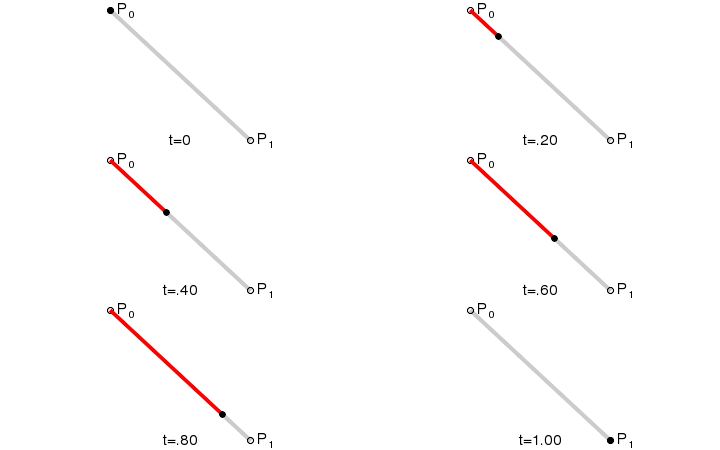
In order to understand higher order Bezier curves, let’s start with the simplest, the line. Graphically, a Bezier line can be generated by linerarly moving between the endpoints, as seen in the image to the right. Algebraically, we can write this as:
\begin{equation*}
L = (1-t)P_0 + tP_1
\end{equation*}

Subsubsection 5.2.2.2 Bezier Quadratic
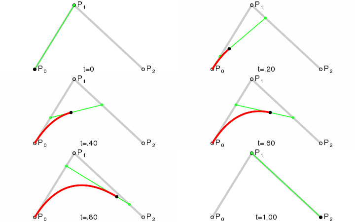
A quadratic needs one more point than the line. This creates 2 normal lines, that we move along in the standard fashion. This creates a series of endpooints that we can use to create a new line (pictured in green). As we move along each static line, we also move along the dynamic line, which in turn generates the points on our quadratic curve. Since the quadratic is generated by moving across a line, we could represent it as:
\begin{equation*}
Q = (1-t)L_0 + tL_1
\end{equation*}
But \(L_1, L_0\) are not points, they’re lines. Substituting in the linear equation, we get:
\begin{equation*}
\begin{aligned}
Q \amp= (1-t)[(1-t)P_0+tP_1] + t[(1-t)P_1+tP_2] \\
Q \amp= (1-t)^2P_0 + t(1-t)P_1 + t(1-2)P_1 + t^2P_2 \\
Q \amp= (1-t)^2P_0 + 2t(1-t)P_1 + t^2P_2
\end{aligned}
\end{equation*}

Subsubsection 5.2.2.3 Bezier Cubic
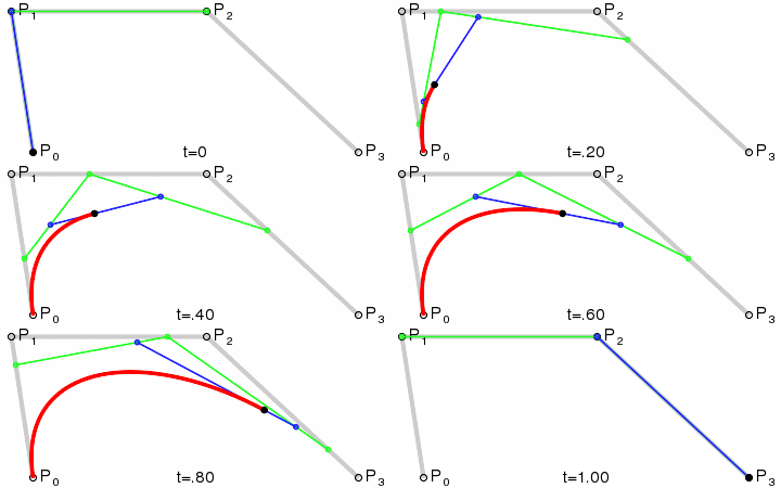
Just as a quadratic is made from 2 linear bezier cuves, a cubic is generated by moving along a line whose endpoints would generate 2 quadratic curves. The blue line generates the cubic, and its endpoints march along the green lines, which in turn march along the staic gray lines connecting all the input points. Since the cubic is generated by moving across a line, we could represent it as:
\begin{equation*}
C = (1-t)Q_0 + tQ_1
\end{equation*}
But \(Q_1, Q_0\) are not points, they’re quadratics! Substituting in the quadratic bezier equations is a bit uglier, though the keen observer may have noticed these equations follow the binomial expansion...
\begin{equation*}
\begin{aligned}
C \amp= (1-t)[(1-t)^2P_0 + 2t(1-t)P_1 + t^2P_2] + t[(1-t)^2P_1 + 2t(1-t)P_2 + t^2P_3] \\
C \amp= (1-t)^3P_0 + 3t(1-t)^2P_1 + 3t^2(1-t)P_2 + t^3P_3
\end{aligned}
\end{equation*}

Subsubsection 5.2.2.4 Bezier Implementation
Now we have an equation \(C\text{,}\) that will generate points along a cubic Bezier curve, but \(t\) is spread throughout the equation. With a little more algebra we can get to:
\begin{equation*}
C = (-P_0 + 3P_1 - 3P_2 + P_3)t^3 + (3P_0 - 6P_1 + 3P_2)t^2 + (-3P_0 + 3P_1)t + P_0
\end{equation*}
This is a cubic of the form \(at^3 + bt^2 + ct + d\text{,}\) that we can put into a parametric loop, the same way we generated Hermite curves. In fact, if we wanted to, we could use our existing matrix multiplication framework to generate the coeficients based on the given information (this is not a necessary step)
\begin{equation*}
\begin{array}{c}
B \\
\left[
\begin{matrix} -1 \amp 3 \amp -3 \amp 1
\\\ 3 \amp -6 \amp 3 \amp 0
\\\ -3 \amp 3 \amp 0 \amp 0
\\\ 1 \amp 0 \amp 0 \amp 0
\end{matrix}
\right]
\end{array}
\begin{array}{c}
G \\
\left[
\begin{matrix} P_0
\\\ P_1
\\\ P_2
\\\ P_3
\end{matrix}
\right]
\end{array}
=
\begin{array}{c}
\\
\left[
\begin{matrix} -P_0 + 3P_1 - 3P_2 + P_3
\\\ 3P_0 - 6P_1 + 3P_2
\\\ -3P_0 + 3P_1
\\\ P_0
\end{matrix}
\right]
\end{array}
=
\begin{array}{c}
C \\
\left[
\begin{matrix} a
\\\ b
\\\ c
\\\ d
\end{matrix}
\right]
\end{array}
\end{equation*}
