Chapter 4 Transformations
Section 4.1 Transformation Matrices
In order to perform transformations, we will construct a transformation matrix \(F\text{,}\) which can then be applied to our edge matrix \(E\) by matrix multiplication. By asserting that the order of multiplication is always \(FE\text{,}\) we can constrain \(F\) to always be a \(4\times4\) matrix. For each transformation, it is helpful to think of it with the following framework:
- What information is required in order to perform the transformation?
- What happens to \((x, y, z)\) after the transformation is applied?
While there are many transformations we could create, we will focus on translation, dilation, and rotation for our graphics engine. These will allow us to make interesting manupulations of our images, while also demonstrating how to develop other transformations, if desired.
Subsection 4.1.1 Translation
Translations can be thought of as sliding an image along any axis. Translations should preserve the number of points, the order of the points, as well as the distances between them.
- Necessary information: Translation factors for each component, \((a, b, c)\)
- Function: \(T_{a, b, c} (x, y, z) \rightarrow (x+a, y+b, z+c)\)
You can generate a translation matrix by starting with the Identity matrix, and then replacing the values in the last column with your translation factors like so:
\begin{equation*}
\begin{bmatrix} 1 \amp 0 \amp 0 \amp a
\\\ 0 \amp 1 \amp 0 \amp b
\\\ 0 \amp 0 \amp 1 \amp c
\\\ 0 \amp 0 \amp 0 \amp 1
\end{bmatrix}
\begin{bmatrix} x_0 \amp x_1
\\ y_0 \amp y_1
\\ z_0 \amp z_1
\\ 1 \amp 1\end{bmatrix} =
\begin{bmatrix} x_0 + a \amp x_1 + a
\\y_0 + b \amp y_1 + b
\\z_0 + c \amp z_1 + c
\\ 1 \amp 1 \end{bmatrix}
\end{equation*}
Note that this simple translation matrix is made possible by including the bottom row of 1s in our edge matrix. Without that, we’d have to include operations like: \(\dfrac{x + a}{x}\text{,}\) which would in turn mean that the translation matrix would have to change for every point in the edge matrix, like so:
\begin{equation*}
\begin{bmatrix} \frac{x_0+a}{x_0} \amp 0 \amp 0
\\\ 0 \amp \frac{y_0+b}{y_0} \amp 0
\\\ 0 \amp 0 \amp \frac{z_0+c}{z_0}
\end{bmatrix}
\begin{bmatrix} x_0
\\ y_0
\\ z_0 \end{bmatrix} =
\begin{bmatrix} x_0 + a
\\y_0 + b
\\z_0 + c\end{bmatrix}
\end{equation*}
Subsection 4.1.2 Dilation
Dilation (or scaling) is enlarging or shrinking an image. Dilations will preserve the number and order of points, but not the distance (unless the dilation factor is 1 for all coordinates). Currently, dilations will be performed with respect ot the origin, meaning that objects not centered at the origin will also move away (when enlarging) or toward (when shrinking) the origin. Eventually, this will be less of a concern, but for now, you can achieve arbitrary dilations by translating to the origin, dilating, and then translating back.
- Necessary information: Dilation factors for each component, \((a, b, c)\)
- Function: \(D_{a, b, c} (x, y, z) \rightarrow (ax, by, cz)\)
You can generate a dilation matrix by starting with the Identity matrix, and then replacing the 1s with your translation factors like so:
\begin{equation*}
\begin{bmatrix} a \amp 0 \amp 0 \amp 0
\\\ 0 \amp b \amp 0 \amp 0
\\\ 0 \amp 0 \amp c \amp 0
\\\ 0 \amp 0 \amp 0 \amp 1
\end{bmatrix}
\begin{bmatrix} x_0 \amp x_1
\\ y_0 \amp y_1
\\ z_0 \amp z_1
\\ 1 \amp 1
\end{bmatrix} =
\begin{bmatrix} ax_0 \amp ax_1
\\by_0 \amp by_1
\\cz_0 \amp cz_1
\\ 1 \amp 1
\end{bmatrix}
\end{equation*}
Dilations intended to preserve the asptect ratio of the orginal image should use the same value for \(a\text{,}\) \(b\text{,}\) and \(c\text{.}\) Using different values will resulting in stretching/squishing the image in verious dimentions.
Subsection 4.1.3 Rotation
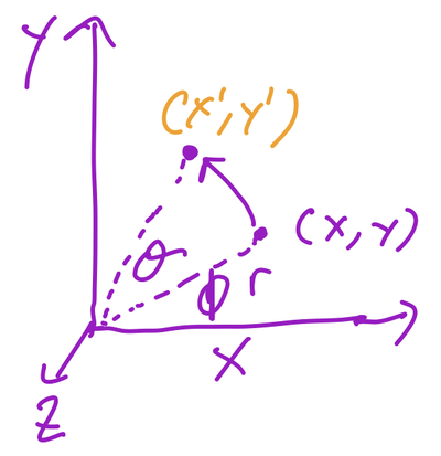
Like dilations rotations will also be performed with respect to the origin. We will be performing 2D rotations in 3D space. So for any rotation, one coordinate will remain fixed, and the others will change based on the rotation. We will refer to the fixed coordinate as the axis of rotation.
Figuring out the rotation function is a bit more complicated than the previous transformations. First let’s look at a rotation about the z axis:  Since the point does not change along the axis of rotation, we only need to conern ourselves with \((x, y)\) We need to find a way to represent \((x',y')\) based on information we know. Using polar coordinates, we can re-write \((x, y)\) as \((rcos\phi, rsin\phi)\) Similarly, \((x', y')\) can be written as \((rcos(\phi+\theta), rsin(\phi+\theta))\) Using the angle sum formula, and the values for \((x, y)\) above, we get the following:

\begin{equation*}
x' = rcos(\phi + \theta) \quad y' = rsin(\phi + \theta)
\end{equation*}
\begin{equation*}
x' = rcos\phi cos\theta - rsin\phi sin\theta \quad y' = rsin\phi cos\theta + rcos\phi sin\theta
\end{equation*}
\begin{equation*}
x' = xcos\theta - ysin\theta \quad y' = ycos\theta + xsin\theta
\end{equation*}
This gives us \((x', y')\) in terms of values we know. Because rotations change depending on the fixed axis, we will have 3 different rotation functions.
- Necessary information: Angle of rotation, \(\theta\) and axis of rotation.
- Function: See below for each axis of rotation
Subsubsection 4.1.3.1 Z-Axis Rotation
Function: \(R_{\theta, z-axis} (x, y, z) \rightarrow (xcos\theta-ysin\theta, xsin\theta+ycos\theta,z)\)
\begin{equation*}
\begin{bmatrix} cos\theta \amp -sin\theta \amp 0 \amp 0
\\\ sin\theta \amp cos\theta \amp 0 \amp 0
\\\ 0 \amp 0 \amp 1 \amp 0
\\\ 0 \amp 0 \amp 0 \amp 1
\end{bmatrix}
\begin{bmatrix} x_0
\\ y_0
\\ z_0
\\ 1
\end{bmatrix} =
\begin{bmatrix} x_0cos\theta-y_0sin\theta
\\x_0sin\theta + y_0cos\theta
\\z_0
\\ 1
\end{bmatrix}
\end{equation*}
Subsubsection 4.1.3.2 X-Axis Rotation
Function: \(R_{\theta, x-axis} (x, y, z) \rightarrow (x, ycos\theta - zsin\theta, ysin\theta + zcos\theta)\)
\begin{equation*}
\begin{bmatrix} 1 \amp 0 \amp 0 \amp 0
\\\ 0 \amp cos\theta \amp -sin\theta \amp 0
\\\ 0 \amp sin\theta \amp cos\theta \amp 0
\\\ 0 \amp 0 \amp 0 \amp 1
\end{bmatrix}
\begin{bmatrix} x_0
\\ y_0
\\ z_0
\\ 1
\end{bmatrix} =
\begin{bmatrix} x_0
\\y_0cos\theta - z_0sin\theta
\\y_0sin\theta + z_0cos\theta
\\ 1
\end{bmatrix}
\end{equation*}
Subsubsection 4.1.3.3 Y-Axis Rotation
Function: \(R_{\theta, y-axis} (x, y, z) \rightarrow (xcos\theta+zsin\theta, y, -xsin\theta + zcos\theta)\)
\begin{equation*}
\begin{bmatrix} cos\theta \amp 0 \amp sin\theta \amp 0
\\\ 0 \amp 1 \amp 0 \amp 0
\\\ -sin\theta \amp 0 \amp cos\theta \amp 0
\\\ 0 \amp 0 \amp 0 \amp 1
\end{bmatrix}
\begin{bmatrix} x_0
\\ y_0
\\ z_0
\\ 1
\end{bmatrix} =
\begin{bmatrix} x_0cos\theta+z_0sin\theta
\\y_0
\\-x_0sin\theta + z_0cos\theta
\\ 1
\end{bmatrix}
\end{equation*}
Section 4.2 Combining Transformations
Let’s say we have the following matrices:
- \(E_0\text{:}\) Edge matrix
- \(T\text{:}\) Translation
- \(D\text{:}\) Dilation
- \(R\text{:}\) Rotation
And we perform the following operations to generate new edge matrices:
- \(E_1 = TE_0\text{:}\) \(E_0\text{,}\) moved
- \(E_2 = DE_1\text{:}\) \(E_0\text{,}\) moved, then scaled
- \(E_3 = RE_2\text{:}\) \(E_0\text{,}\) moved, then scaled, then rotated
Substituting back up the chain we get:
\begin{equation*}
\begin{aligned}
E_3 \amp= RE_2 \\
E_3 \amp= R(DE_1) \\
E_3 \amp= R(D(TE_0))
\end{aligned}
\end{equation*}
Or more clearly, \(E_3 = RDTE_0\text{.}\) Becuse matrix multiplication is associative, we can write this as
\begin{equation*}
E_3 = (RDT)E_0
\end{equation*}
Which means that we can generate the same image by multipling transformation matrices with each other then multiplying by an edge matrix as we could by multiplying the edge matrix by each transformation matrix separately. This could save lots of time, since all transformation matrices are \(4\times4\text{,}\) while our edge matrices are \(4\times N\text{.}\)
The order is important. Note that:
\begin{equation*}
(RDT)E_0
\end{equation*}
is not the same as
\begin{equation*}
(TDR)E_0
\end{equation*}
because matrix multiplication is not commutative. The first image would be the reslut of moving, scaling, then rotating. The second would be the result of rotating, scaling, then moving. It is common (since most of us are used to reading left->right), to think about the appilcation of transformations that way. You have been warned.
