Chapter 10 Scanline Conversion
Section 10.1 Overview
Scanline conversion is the process of filling in a polygon by drawing a series of horizontal (or vertical) lines covering the entire surface of the polygon. This has a number of advantages over other possible approaches such as:
- The y value for each scanline is just 1 plus the previous y value.
- Horizontal lines have the same y value for each pixel, negating the need for y calculations inside the line algorithm.
- We can cover the entire surface while only visiting each pixel exactly once
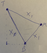
In order to scanline convert a triangle, the first thing we have to do is find the top, bottom and middle vertices. As long as each triangle in our triangle matrix has 3 distinct vertices, there will always at least be a distinct top and bottom (this is why it was important not to add the degenerate triangles at the poles of a sphere). We can define the middle as the vertex that isn’t either the top or bottom (more on this later). After ordering our vertices vertically, we have something like this: 

Section 10.2 Scanlines
Each scanline will go from one edge of the triangle to another. In order to draw each line, we have to determine the endpoints. \(y\) values are very simple. They start at the bottom (\(y_b\)), go up by 1 each time, and end at the top (\(y_t\)). The \(x\) values are more complicated. They must move along the edges of the triangle. In the diagram above, I’ve designated that \(x_0\) for each scanline to be the endpoint somewhere along the line \(\overline{BT}\text{,}\) and \(x_1\) will be the other endpoint, which will either be along \(\overline{BM}\) or \(\overline{MT}\text{,}\) depending on how far up we’ve made it. It doesn’t matter if the middle vertex is to the left of right of the \(\overline{BT}\) edge, since our
draw_line function will swap endpoints if they’re not listed left to right. This will make it easier to develop the scanline algorithm.Subsection 10.2.1 Calculating \(x_0\)
\(x_0\) starts at \(x_b\) and ends at \(x_t\text{.}\) The question is, how much does \(x_0\) change with each scanline (\(\Delta x_0\))? The total change in \(x_0\) is \(x_t - x_b\text{,}\) which occurs over the course of drawing each scanline. So the number of scanlines determines the number of times we change \(x_0\text{.}\) In turn, the number of scanlines is just the difference in \(y\) over the course of the triangle.
\begin{equation*}
\Delta x_0 = \frac{x_t - x_b}{y_t - y_b + 1}
\end{equation*}
(we need to add 1 to the y difference to account for the bottom-most line).
Subsection 10.2.2 Calculating \(x_1\)
\(x_1\) also starts at \(x_b\text{,}\) but it ends at \(x_m\) and then changes direction to go towards \(x_t\text{.}\) We need to calculate \(\Delta x_1\) similarly to how we calcluated \(x_0\text{,}\) but we will have 2 different values, depending on whether we’ve moved past the middle vertex or not.
\begin{equation*}
\begin{aligned}
\Delta x_1 = \frac{x_m - x_b}{y_m - y_b + 1} \\
\Delta x_1 = \frac{x_t - x_m}{y_t - y_m + 1}
\end{aligned}\text{.}
\end{equation*}
We flip from the first to the second calculation once our \(y\) has reached \(y_m\text{.}\)
Section 10.3 The Algorithm
Putting this all together, we can come up with this pseudocode outline:
        //initial setup, find b, t, m
        x0 = xb, x1 = xb, y0 = yb
        dx0 = (xt - xb) / (yt - yb)
        dx1 = (xm - xb) / (ym - yb)
        dx1_1 = (xt - xm) / (yt - ym)
        while y <= yt
            draw_line(x0, y, x1, y)
            //move the endpoints
            x0+= dx0
            x1+= dx1
            y+= 1
            //swap dx1 if neeced
            if y >= ym
                dx1 = dx1_1
                x1 = xm
It is a good idea to think of the loop here as having 3 distinct parts:
- drawing the line
- updating the endpoints
- swapping \(\Delta x_1\)
The order in which you do these may not match the outline above, depending on how you handle "special" cases and other potential issues as they arise.
Subsection 10.3.1 "Special" Triangles
Scanline conversion works very well when there are distinct top, bottom and middle vertices. Sometimes, there is no distinct middle (once again, there will always be a top and bottom). These are cases when two vertices have the same \(y\) value (either the top or bottom is a flat horizontal line). But the \(x\) values will be different, which is important. You can handle these cases either explicitly or implicitly, but you do need to consider them.
